| |
Experimental Hydrometeorology Laboratory |
Welcome to this web page built and maintained by the Experimental Hydrometeorology Laboratory of the Federal University of Rio de Janeiro (lhydex-UFRJ).
Our laboratory investigates the water cycle in the atmosphere and on the Earth's surface. We contribute to training high-level technical personnel in hydrometeorology, enabling them to understand the role of water in the Earth's climate system. We provide an excellent research environment for undergraduate (scientific initiation) and graduate students (master's and doctoral), preparing them to analyze environmental and technological risks in today's society.
Additionally, we maintain scientific collaborations with researchers from other institutions and welcome postdoctoral proposals. In the realm of education, we collaborate on disciplines covering hydrometeorology, weather radar, urban meteorology, environmental disasters, natural hazards, and resilience.
If you are interested in Science, Technology, Engineering, and Mathematics (STEM), you are welcome to join us in scientific initiation or postgraduate research projects.
The Laboratory is coordinated by Prof. Hugo Abi Karam.
Introduction
This webpage provides a comprehensive overview of hydrometeorological hazard modeling and risk assessment outcomes. The system integrates various numerical models, including:
- A hydrological model with variational assimilation for heterogeneous forcings.
- A representation of surface water transport.
- A subsurface model.
- A landslide model.
- A river flood model.
- Atmospheric optical flow techniques for immediate storm prediction based on rainfall field advection.
Precipitation estimates, derived from satellite data (space-time distribution field), facilitate the assessment of landslide and river flooding probabilities. These assessments involve analyzing the temporal and spatial evolution of logistic probability distributions of hazards across regional topography and soil with varying moisture levels
The hydrological model assimilates atmospheric precipitation fields to determine water distribution in the soil's upper layer, and a path model facilitates the movement of surface water (non-infiltrated water) to rivers.
The landslide model calculates the conditional factor of safety for moistened soil using a logistic probability distribution function to track landslide evolution. Additionally, a river section model, based on trapezoidal stream sections, estimates river water levels to evaluate overflow risks on floodplains.
Optical flow techniques are employed to advect thunderstorm rainfall fields, enabling short-term forecasting up to three hours ahead with 15-minute intervals. Results are visualized as a movie with frames at 15-minute intervals, and each frame is verified against previous results.
These factors contribute to a risk model, defined as the product of hazard conditional probability, population exposure, and vulnerability. In risk-prone areas, such as Brazilian hillsides or floodplains, the terms hazard and risk are often used interchangeably. However, hazard implies a potential threat, while risk encompasses management and mitigation measures for vulnerable areas. Risk can range from tolerable to catastrophic, depending on the control measures implemented.
Atmospheric precipitation data from the Hydro-Estimator/NOAA satellite drive these models. A digital surface elevation model, such as SRTM/NASA data, defines boundary conditions. Water balance assessments evaluate surface soil stability and moisture content, which are crucial for understanding hydrometeorological hazards such as floods and landslides. Outputs, including conditional probability distributions for landslides and floods, inform risk assessments and managerial decisions in regional contexts.
Initially applied in Rio de Janeiro and surrounding areas, future iterations may expand to other regions. Current versions incorporate rainfall data from across South America.
Content outline
- A series of variables related to the risk of hydrometeorological hazards, such as the precipitation rate [r] in (mm/h), accumulated precipitation [R] in (mm) and various surface and soil hydrological variables ( topographic index, soil cohesion, safety factor, probabilities, etc.) dynamically variable in time and space.
- Informations and Primary Sources:
- Atmospheric precipitation data (Hydroestimator-NOAA);
- Topographic digital data (SRTM-NASA);
- Numerical codes, programs and scripts (for linux) are original and available at lhydex-UFRJ;
- Results of the dynamic hydrometeorological hazards model and advective nowcasting are updated in short cycles (full refresh every 15 minutes);
- Graphical results of the model (plots and animations) were made available by the Laboratory of Experimental Hydrometeorology of the Federal University of Rio de Janeiro - UFRJ, unless otherwise indicated;
- How to interpret the results?
- Disclaim statement.
- References.
Updating charts
The current site version is automatically updated every 300 seconds (5 minutes), with no user intervention required.
If you want to force an update at any time, please follow these instructions: To refresh the display of site graphics (i.e., overwrite cached content), press Ctrl+R (Ctrl+Alt+R), Ctrl+Fn+F5, or Ctrl+F5, depending on your keyboard and OS. On mobile devices, use incognito mode to automatically update the pages as they are opened.
The graph set is completely refreshed every 15 minutes on the current computer system.
Numerical formulation
The computational system, proxy of the risk model, has the following coupled main components (each one containing scripts, programs and subroutines):
- dataset/mycron.sh [chronometer and jobs launching] (sh)
- hydromet_risk_v*.* [input data preparation] (f90)
- TopModel_variational_f90_v*.* [hydrological model] (f90)
- landslide_model*.* [hazard model] (f90)
- surface_flow_routing*.* [path model] (f90)
- river_outflow_model*.* [hazard model] (f90)
- optical_flow*.* [nowcasting preparation] (f90)
- nowcasting_advection*.* (f90)
- model_skill_evaluation*.* (f90)
- Graphics were obtained with grads and gnuplot.
We are continuously improving the codes and routines to avoid interruptions (using try and catch procedures).
The Digital Elevation Model of the SRTM (Rodriguez et al. 2005; Farr et al. 2007) is used in the present hydrological models, providing a nominal resolution up to 90 m.
The grafics and figures shown above were obtain by use of the scripts: dataset/mycron.sh (hydroestimator.sh + graphics.sh + mysite.sh)] plus the numerical program TopModel_variational (gfortran, f90) in the plaform environment linux (Ubuntu).
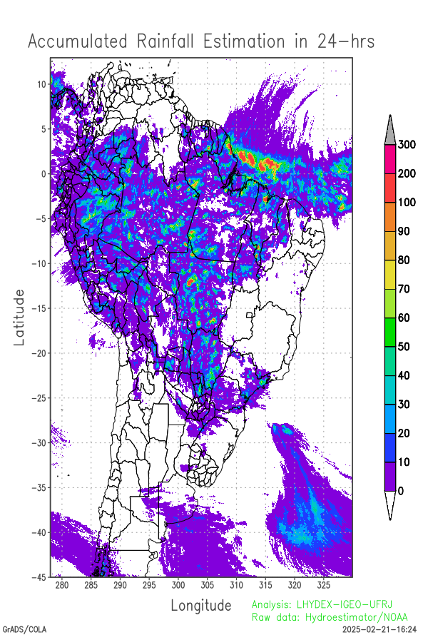
Precipitation Estimation for South America
Rainfall [r] in (mm h-1) and Accumulated Rainfall [R] in (mm). Primary data source: web link
The graphical and animations results shown on this page are computational research products made available by the Laboratory of Experimental Hydrometeorology (lhydex-UFRJ) of the Federal University of Rio de Janeiro, unless otherwise indicated.
The update date is present in the lower right corner of many of the plots. Date and time shown in the figures corresponds to Brasília Local Time (LT), where LT = UTC-3 hrs, where UTC is the Universal Time Coordinated (Greenwich Mean Time, GMT=UTC+0).
Service interruptions may occur because web servers are subject to maintenance periods. Therefore, continuity is not guaranteed. If you have any questions, please contact the lhydex-UFRJ laboratory coordination. The automatic updating of the website is discontinued when access to Hidroestimator data is interrupted for maintenance of the distribution servers. In general, maintenance periods do not exceed 7 days per year. Maintenance of the lhydex-UFRJ system is generally carried out when the forecast does not indicate rain in RJ. As far as possible, site operation is maintained during all rainy periods, except for maintenance exceptions indicated above.
Dataset analysis:
Last 24-hours of rainfall field evolution (atmospheric forcing):
Soil water distribution for heterogeneous forcing:
The original version of the "TopModel" hydrological model uses a single precipitation time series as a forcing on the underlying hydrological model. Considerations of topographic similarity imply a hydrological distribution associated with topography and its ability to concentrate water flow. Despite its wide use for analyzing distribution in small river basins, its application in larger or regional or continental basins is not recommended precisely due to the lack of heterogeneity in atmospheric and soil surface forcing, which causes variation in infiltration and water distribution.
Among the heterogeneities that can have an impact on the spatial distribution of water in the soil are heterogeneities in the energy and surface water balance, spatial heterogeneities in precipitation and evapotranspiration, distribution of vegetation and surface aerodynamic roughness, presence of impermeable areas such as urban areas, lakes and rivers, heterogeneities in the soil layer, variations in the depth of the water table, hydraulic conductivity, permeability, permittivity, hydraulic diffusivity, variations in soil density, soil moistening effects, variations in the cohesion of soil particles, variations in porosity, variations in the transmissivity of the soil layer, the distribution of soil types in the area, topography, resistance to rupture and movement of the surface layer of soil, variations in slope and resistant friction force and inertia.
To address the common challenges of bulk and semi-distributed models, the assimilation of the variational principle with various heterogeneities has been proposed to generalize the 2-D spatial forcings in hydrological models. This approach yields a distribution that serves as the formal solution to a variational problem, either under weak constraints (based on the mass conservation equation) or strong constraints (based on data assimilation), applied along the Lagrangian paths of water. This is represented by integrating the advection partial differential equation into the variational functional, which adjusts the topographic index while accounting for the evolution of atmospheric forcing.
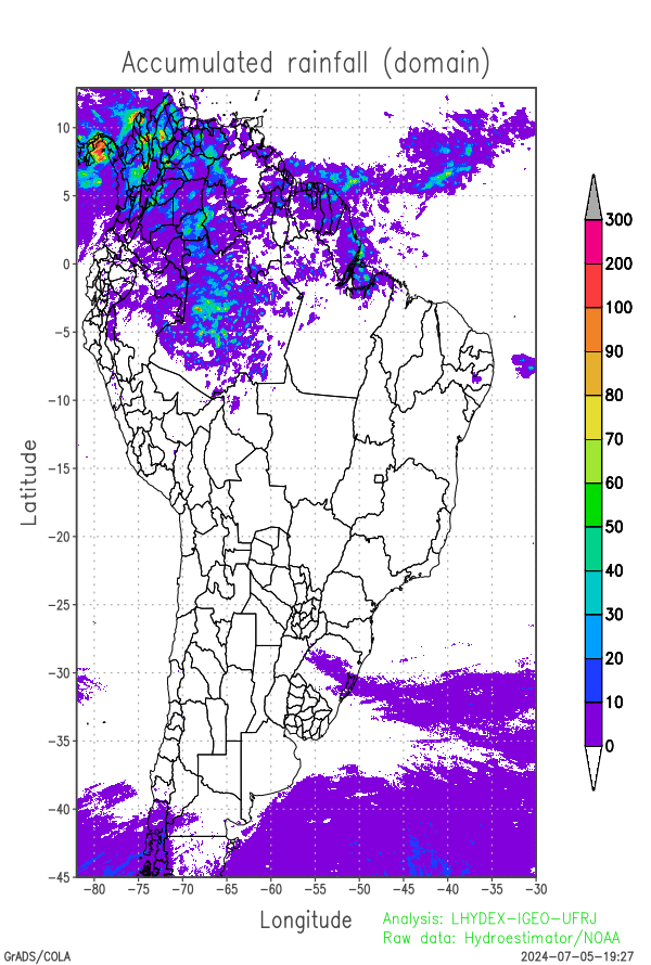
Heteorogeneous forcing: last 24-hrs of rainfall in regional and continental domains:
| Accumulated Rainfall in 24h (mm) (SA domain) (96 frames, images each 15 min) [commands grads] | Accumulated Rainfall in 24h (mm) (SA domain) (96 frames, images each 15 min) [subroutine f90] | Accumulated Rainfall in 24h (mm) (Subdomain) (96 frames, images each 15 min) [subroutine f90] |
|
 |
 |
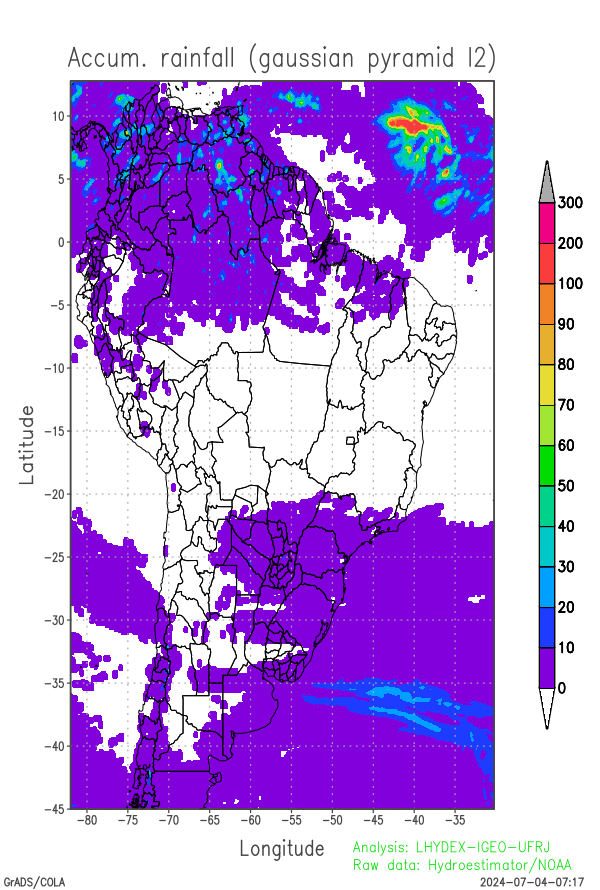
Scale Analysis (Filtered Space):
Gaussian Pyramid (Constructor Method)
The scale analysis is based on obtaining a Gaussian pyramid corresponding to the two-dimensional (f) field, where each level of the pyramid is obtained by applying successive Gaussian filters (from bottom to top), with a progressive reduction in spatial resolution (and the number of grid points). At the end of the pyramid construction, each level can be expanded (by balanced interpolation) until the resolution of the lower levels.
The Gaussian pyramid has (n+1) levels, denoted by g(i), i=0,1,2,3,...,n, with the lower level being equal to the original field (g0 = f). The upper level of the Gaussian pyramid g(n) corresponding to the field that was filtered most times, to show meso alpha-scale and synoptic scale prone risk areas. On the other hand, the lower level corresponds to the original unfiltered field (g0), with all the structure. Small structures are absent in the upper pyramidal level (such as isolated thunderstorms or small groups of thunderstorms). These areas are a proxy for risk areas on a regional scale, which can be refined by the path of storms as they appear in the weather radar field.
Lagrangian Pyramid (Constructor Method)
The Lagrangian pyramid (with n levels) is obtained by subtracting successive levels from the Gaussian pyramid. That is, L(n)=g(n); L(n-1)=g(n)-g(n-1); ...; L1=g2-g1.
The original field can be reconstituted by the sum: f = g1 = L(n) + L(n-1) + ... + L1. Each Lagrangian level maintains, with the exception of the last one L(n), the intermediate scale structure between the successive levels.
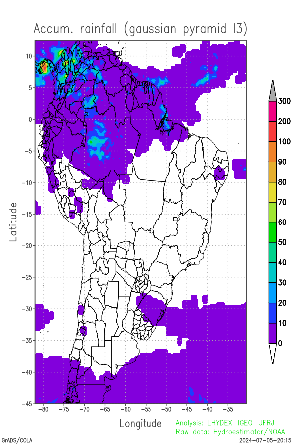
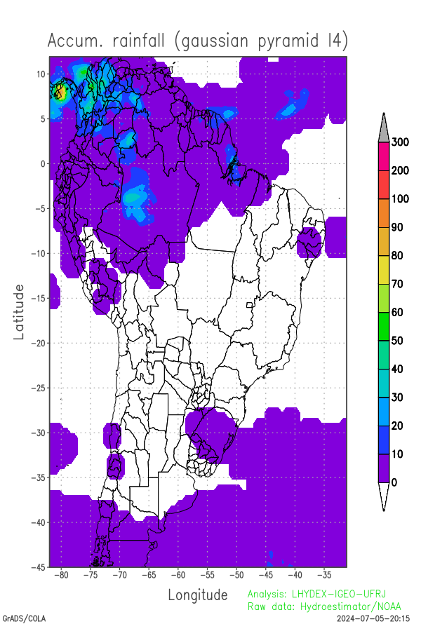
Below are 3 levels of the Gaussian pyramid corresponding to the field of accumulated precipitation over the last 24 hours. In practice, for mapping in South America, only 5 Gaussian levels are sufficient for the transition from the mesoscale structure to the smoothed synoptic scale structures.
| Gaussian Pyramid level of the last 24 hours accumulated rainfall in AS domain (g2) | Gaussian Pyramid level of the last 24 hours accumulated rainfall in AS domain (g3) | Gaussian Pyramid level of the last 24 hours accumulated rainfall in AS domain (g4) |
 |
 |
 |
Radar Reflectivety Parameter [using R-Z relation] (previous 24 hours):
| Animation: Radar: dBZ (-) (last 24 hrs) (Subdom) 2D field with division shapes | Animation: Radar: dBZ (-) (last 24 hrs) (Subdom) 3D surface |
 |
 |
Landslide Model results
Variational TopModel coupled with landslide and flood hazard model (for the previous 24 hours):
As risks are management objects, the word risk is sometimes used in place of the word hazard (event causing danger). However, the definition of risk considers not only the danger, but also the vulnerability of the population, social and environmental susceptibility to exposure to hazards, the degree of governmental and social preparation, etc. Danger comes from a threat. Negligence (carelessness or depreciation), omission and ignorance can place risk events in the danger category.
Assessments of intensity, temporal evolution and probability of hydrometeorological hazards are objectives of a risk management and warning system. In fact, the definition of the risk management system includes other dimensions, in addition to warning of dangers, such as population training programs, social participation in risk management, training for volunteers, training of students at Universities to understand risks, social dissemination, dialogical communication, urbanization and reurbanization, reduction of vulnerabilities, actions in periods of risk and crisis, reforestation, etc.
One of the objectives of a risk analysis and management system is to issue early warnings, whether warnings about landslides on slopes, water overflows from the primary channels of rivers and tributaries, prolonged droughts and droughts, windstorms, tropical cyclones, intense subtropical and extra-tropical cyclones, etc. Specifically, the results of the analysis of the conditions of landslides on slopes and water overflow from the primary channel of rivers and tributaries are presented below. The landslide probability distribution is obtained by estimating the rupture potential of the surface layer of moist soil.
| Animation: cohesion pressure (105 Pa) (Subdomain) | Animation: normal stress (105 Pa) (Subdomain) | Animation: tangent stress (105 Pa) (Subdomain) |
 |
 |
 |
| Animation: resistance force (1012 N) (Subdomain) | Animation: critical precipitation (mm h-1) [critical values ≤ 5] | Animation: saturation deficit (-) (Subdomain) [critical values < 0] |
 |
 |
 |
| Animation: Radar Reflectivity Parameter dBZ = 10 log10(Z/1) (-) (Subdomain) (hail > 60 dBZ) | Animation: Landslide probability variation (%) (% by hour) [critical values > 50%] | Animation: Deficit to rupture (-) (Subdomain) [critical values ~ 0] |
|
 |
 |
| Animation: ln ( topographic index ) (-) (Subdomain) [critical values > 60] | Animation: landslide factor of safety [F] (-) (Subdomain) [critical values ≤ 1] | Animation: critical Precipitation (mm h-1) [what is missing to destabilize] [critical values < 5] |
 |
 |
|
| Animation: volumetric soil wetness (-) (Subdomain) [critical values ≥ 1] | Animation: surface water (mm) ~ (precipitation-infiltration)*time step [critical values ≥ 5 mm] | Animation: contingent landslide probability (%) [critical values ≥ 50%] |  |
 |
 |
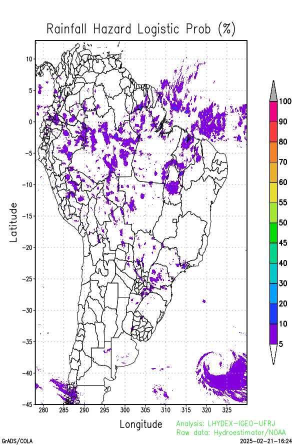
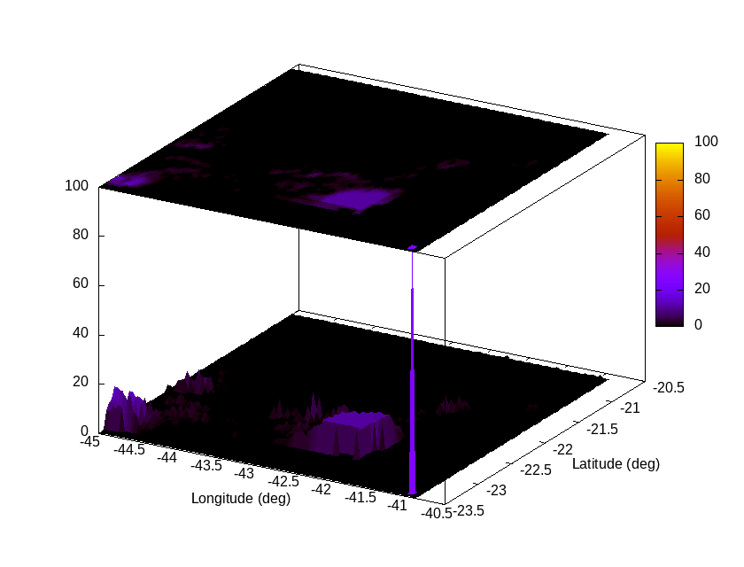
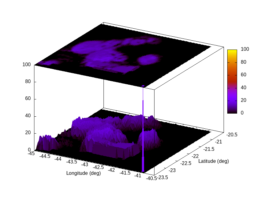
Modeling proxy: distribution of hazard probability (%) (last 3 hours)
| Modeled landslide probability (%) [3D surface map] at analysis time [120 min. ago] (Subdom) | Modeled landslide probability (%) [3D surface map] at analysis time [ 60 min. ago] (Subdom) | Modeled landslide probability (%) [3D surface map] at analysis time [~15 min. ago] (Subdom) |
 |
 |
 |
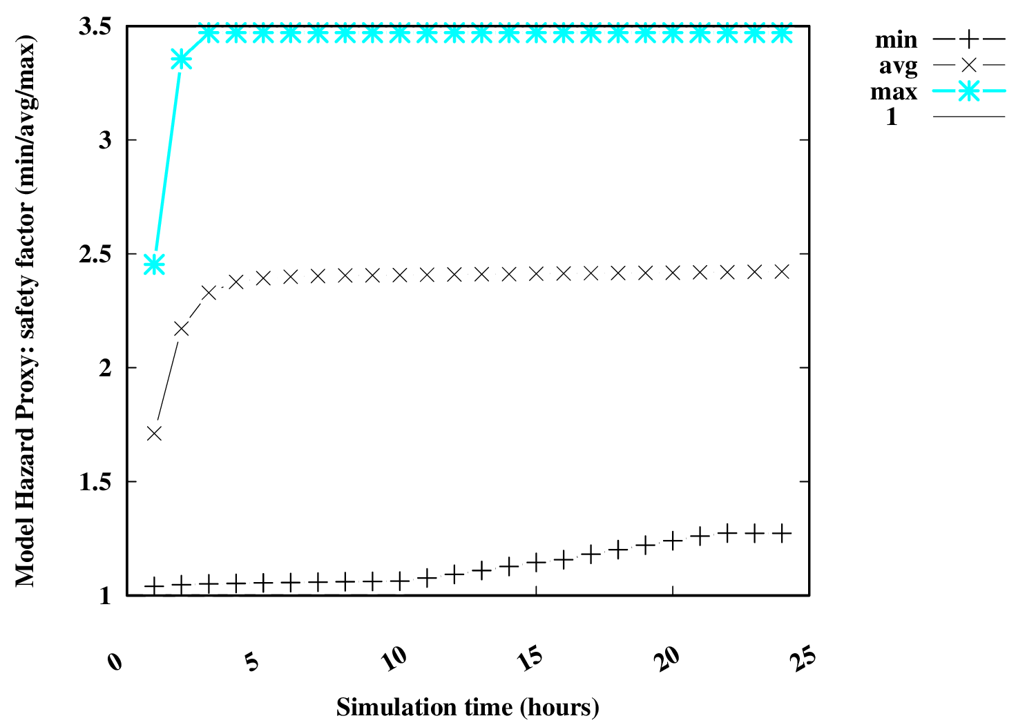
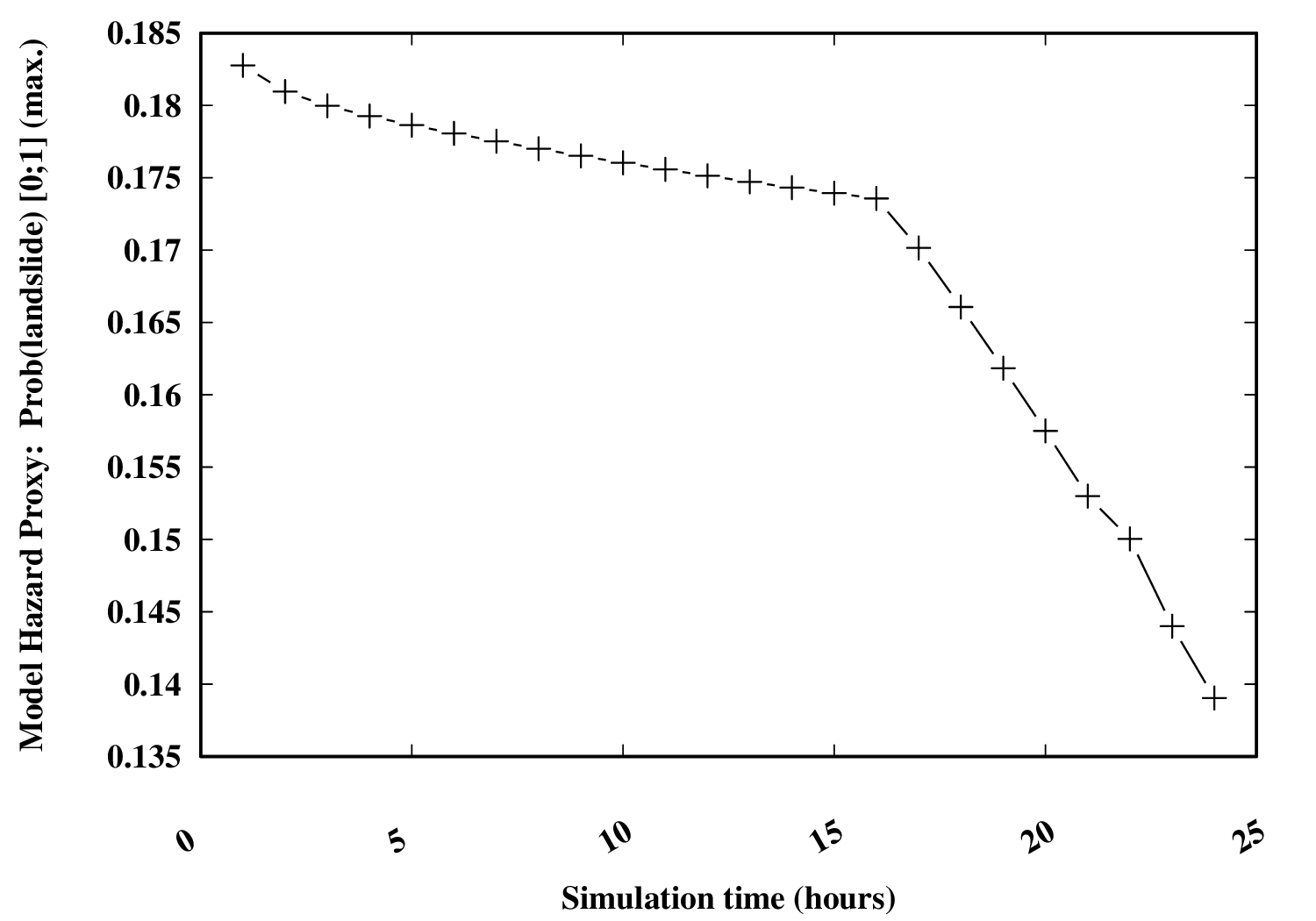
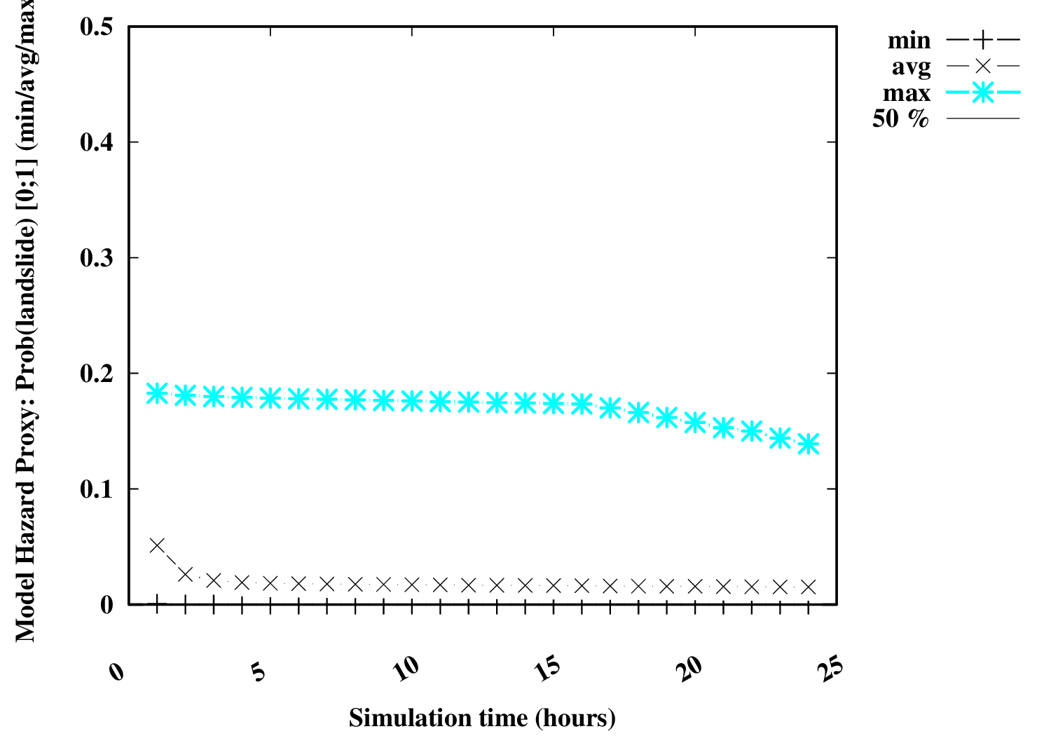
Conditional probability of hidrometeorological hazard evolution (model proxy) [Last 24 hours]
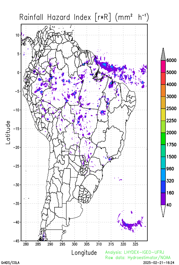
The temporal evolution of the conditional landslide probability can be evaluated by a proxy (i.e., generalized linear regression term), defined by the temporal evolution of the maximum value of the product [r*R] in the spatial domain, at each diagnosis time. This proxy is associated with the temporal variation in precipitation power, as a measure of the evolution of dangerousness, and is given by 1/2*dR2/dt = R*dR/dt = r*R, in units of (mm2 h-1) .
As criteria for defining the alert stage and issuing an alert, fixed thresholds are usually considered: r > rcrit ± σr, R > Rcrit ± σR, or or then use the precipitation intensity evaluated by the product r1h*R24h ≥ (3000 ± 1000) mm2 h-1.
A different approach is to consider the evolution of the temporal variation of the hazard probability, i.e., not just consider the amplitude but also its derivative and conditional curvature over time. This last approach is considered here below. This allows you to assess whether the risk is increasing or decreasing at the present moment, based on its trend and curvature. Particularly, the curvature allows us to infer or anticipate the duration of the process. Increasing trend with small curvature indicates a longer period of exposure to the hazard, while a greater curvature indicates a concentration of the hazard in a short period.
In general, an increasing number of landslides is expected when the conditional probability exceeds the value of 50% (0.5). The greater the margin in relation to 50%, the greater the number of slips expected.
| Geotechnical modeled landslide factor of safety (min/aver/max) [0;3] | Conditional modeled landslide hazard probability: maximum value [0;1] (Subdomain) | Conditional modeled landslide hazard probability: min/aver/max [0;1] (Subdomain) |
 |
 |
 |
| Landslide hazard proxy: maximum rainfall [r] (mm h-1) (Subdomain) | Landslide hazard proxy: maximum accumulated rainfall [R] (mm day-1) (Subdom) | Landslide hazard proxy: maximum periculosity index [r*R] (Subdomain) |
 |
 |
 |
Flood model (with rivers with trapezoidal sections)
Nowcasting the height and water flow of rivers by routing the excess water on the surface in the variational hydrological model
The distribution of surface water (surplus rainfall minus infiltration) allows defining the contribution areas used in routing (transfer of surface water by displacement over the topographic surface to the monitored point of the river). The contribution weight of each area element of the numerical grid is defined by a set of time- and space-dependent linear functions (for heterogeneous precipitation distribution).
The total contributing area is obtained by aggregating the areas of the grid elements intercepted by the trajectories of the water parcels in their downward movement. This occurs as the parcels of surface water travel their trajectory from the source (where there is a surplus of surface water) to the destination at the point of the river, on the advection time scale. The trajectory of many water parcels is obtained by integrating a Lagrangian Particle Model.
The total travel time required for the water parcels to move from their origins to the observation point in the river, along the trajectory following the topography, is obtained from the ratio between the spatial displacement and the surface velocity of the water (obtained from Manning's formulation), segmented along the path.
The wetted area of rivers, streams and canals is a dynamic variable in the surface hydrological model. To establish the relationship between the height of the water and the volumetric flow section, it is necessary to know the cross section of the river. In the proposed model, a trapezoidal cross section is used, embedded in a low-slope gutter. The river channel slopes longitudinally, that is, it slopes along the riverbed. The riverside terrain (banks) also slopes transversely, so that the trapezoidal profile of the river settles into a "V" shaped profile of the terrain on the overbanks. The application of the trapezoidal section of the river is well known in the literature (e.g., Liu et al. 2015).
The base flow of rivers is estimated in the model as a function of the fraction of the average annual precipitation and the catchment area. The river flow gain (average base aquifer flow) for the rainy season is estimated at 32 (mm year-1) or 10-10 (m3 m -2 s-1). Therefore, hourly variations refer only to transient flow disturbances due to rain in the basin in recent hours.
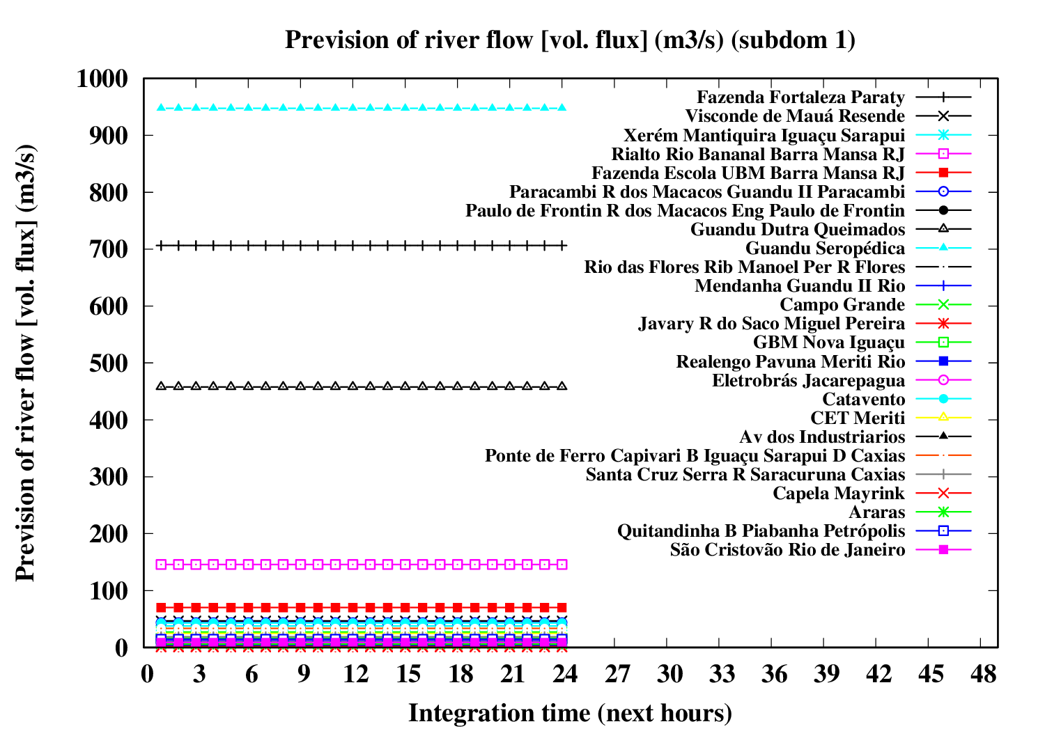
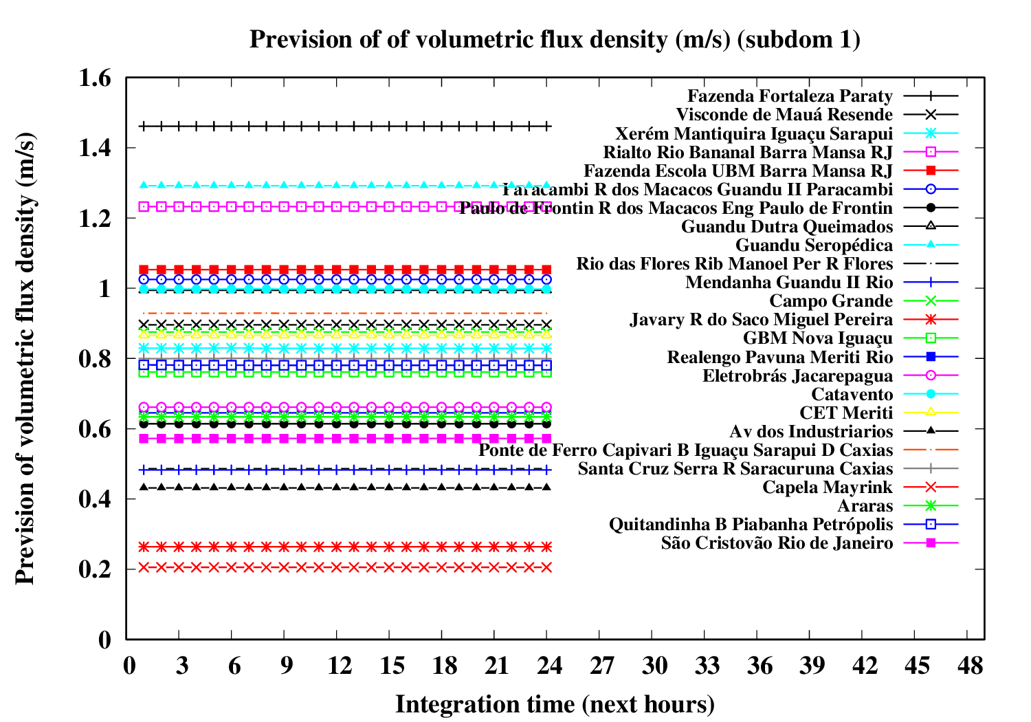
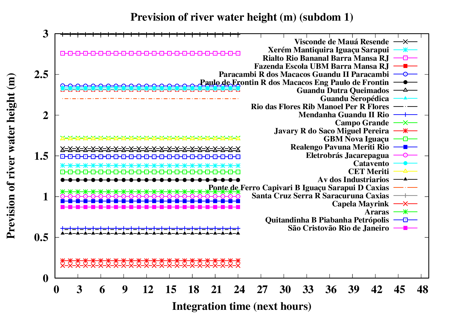
Subdomain 1 (westward):
| a) River water volumetric flux [Q] (m3 s-1) [next 24 hrs] | a) River water volumetric flux density [V] (m s-1) [next 24 hrs] | b) River water heigth [D] (m) [next 24 hrs] |
 |
 |
 |
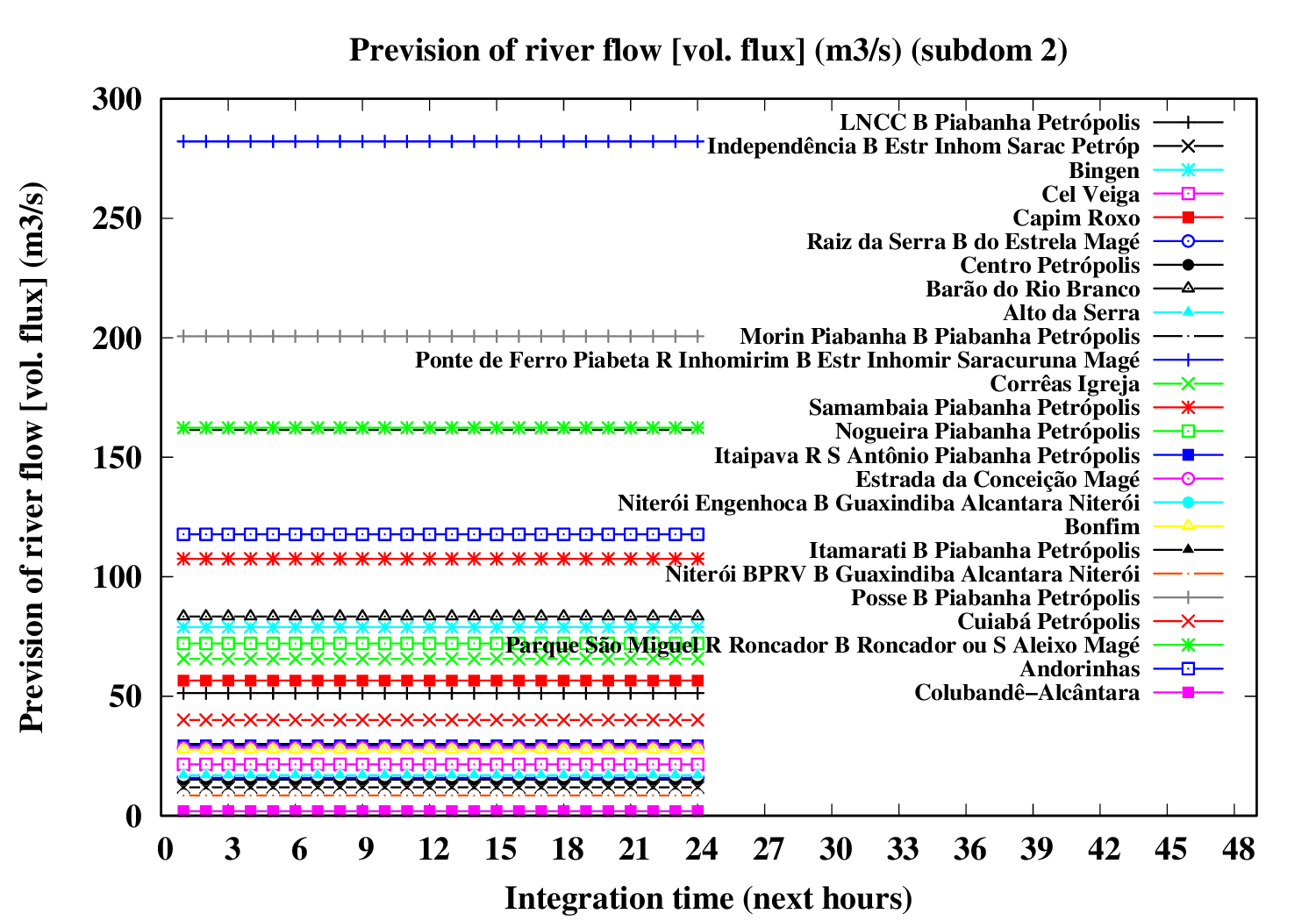
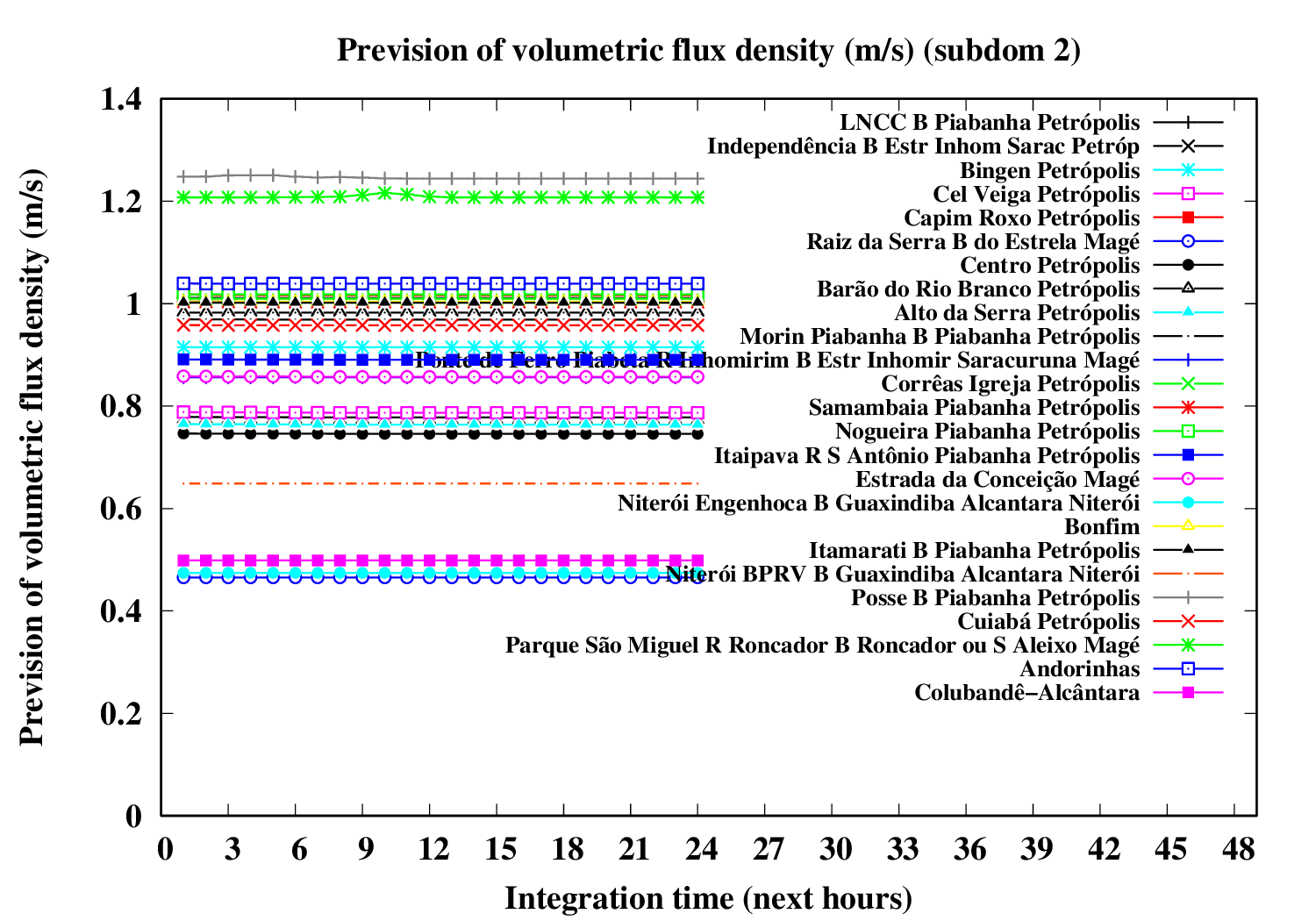
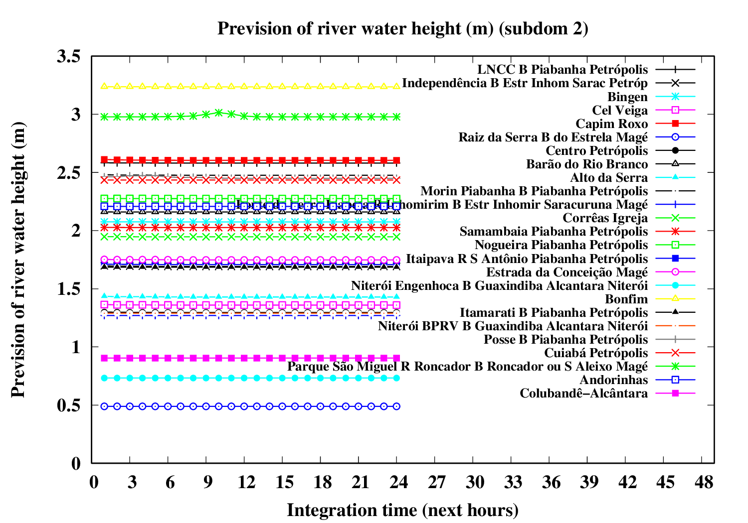
Subdomain 2:
| a) River water volumetric flux [Q] (m3 s-1) [next 24 hrs] | a) River water volumetric flux density [V] (m s-1) [next 24 hrs] | b) River water heigth [D] (m) [next 24 hrs] |
 |
 |
 |
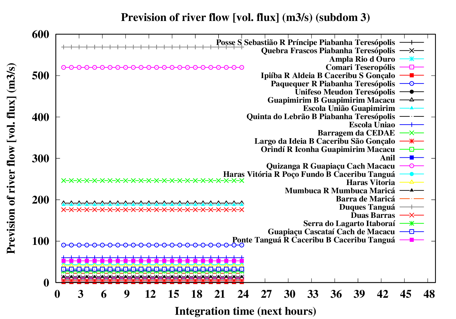
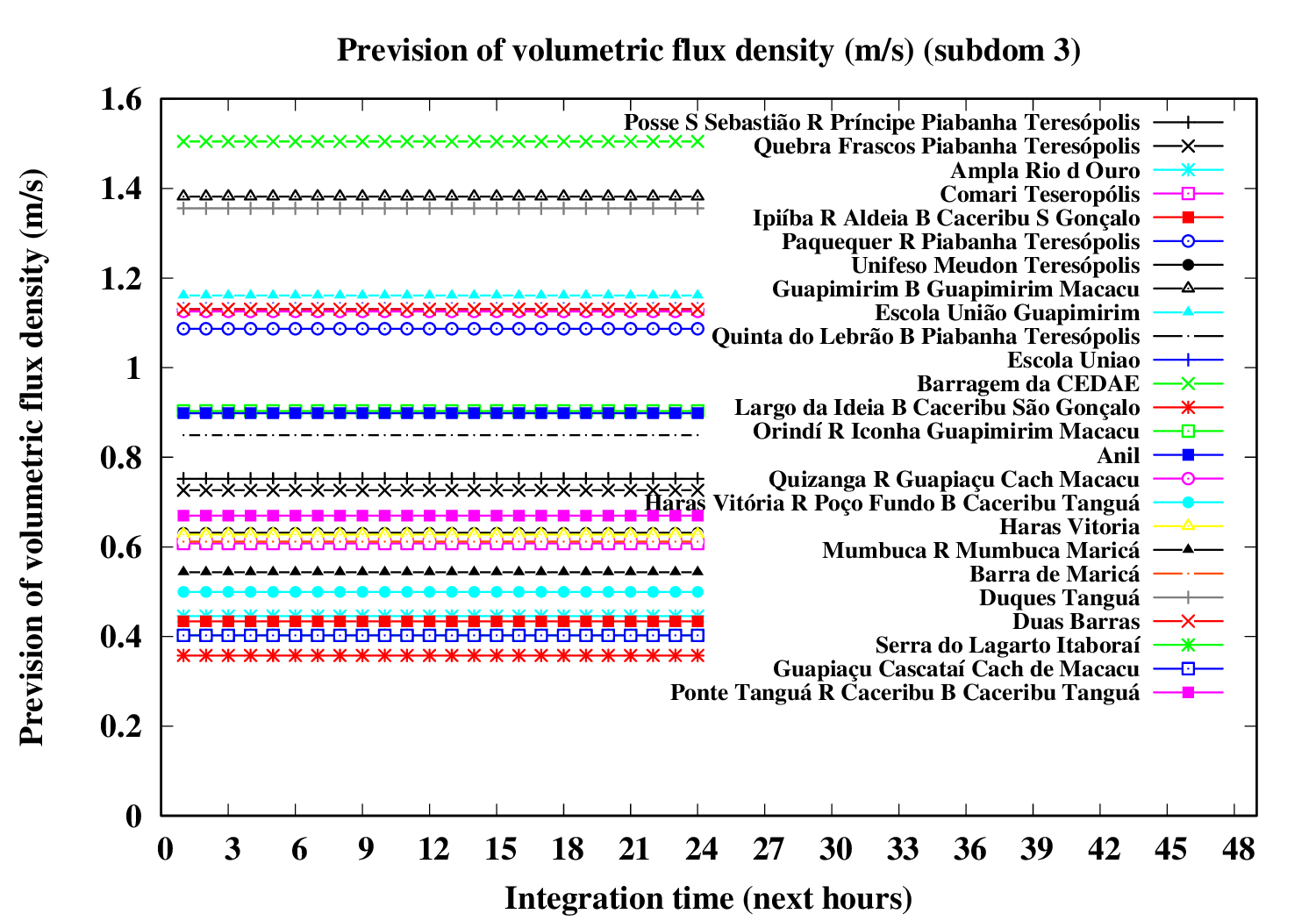
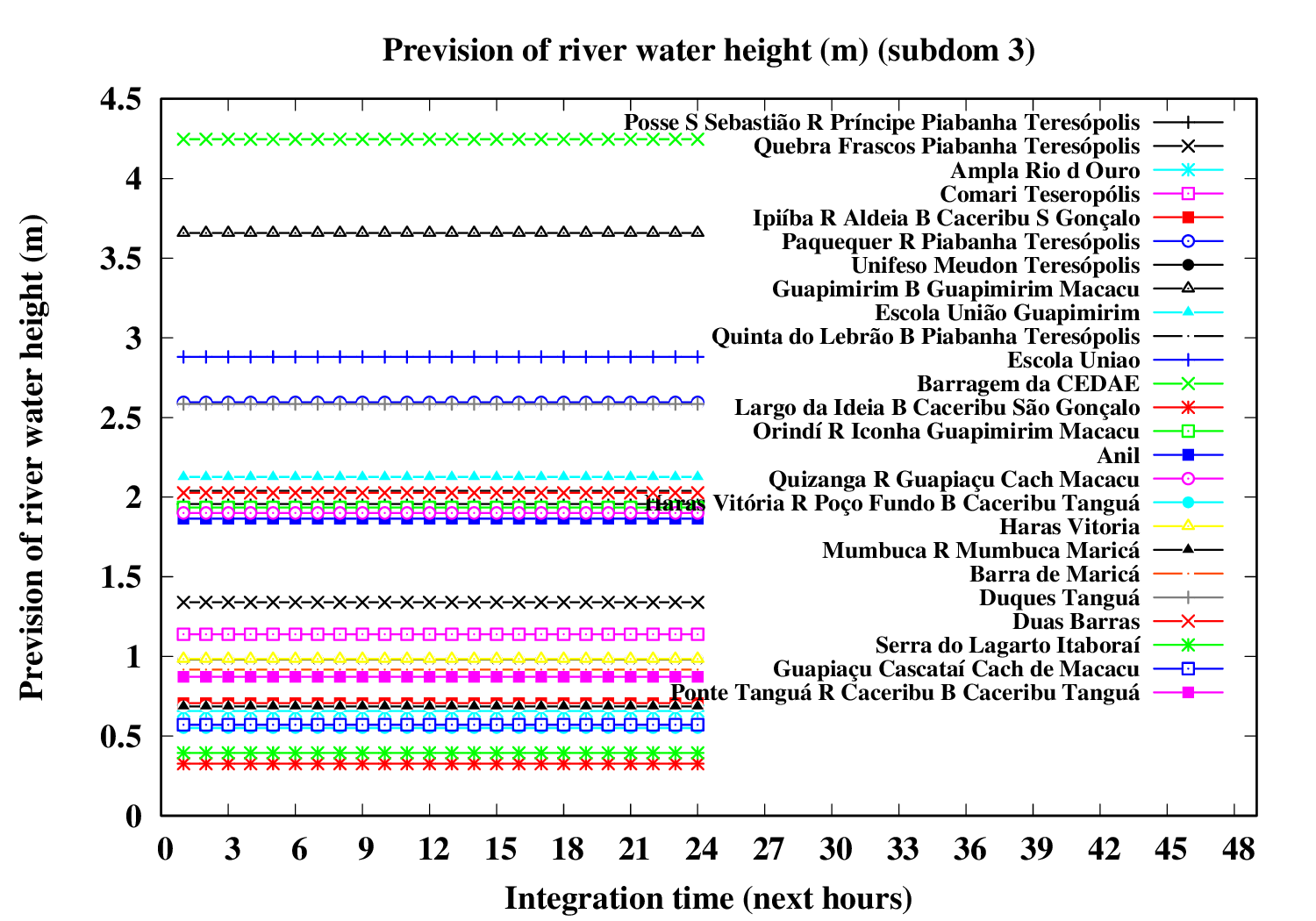
Subdomain 3:
| a) River water volumetric flux [Q] (m3 s-1) [next 24 hrs] | a) River water volumetric flux density [V] (m s-1) [next 24 hrs] | b) River water heigth [D] (m) [next 24 hrs] |
 |
 |
 |
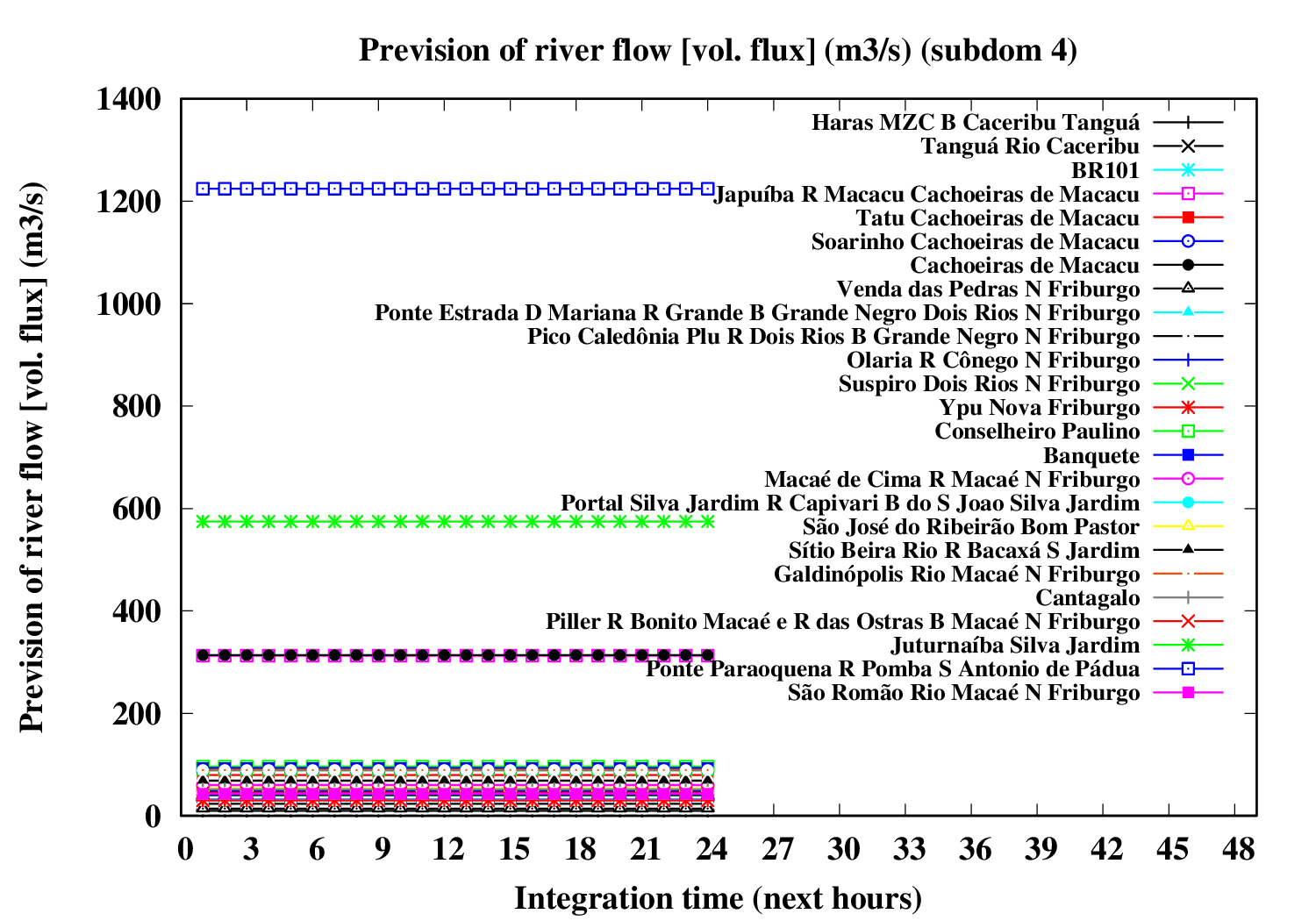
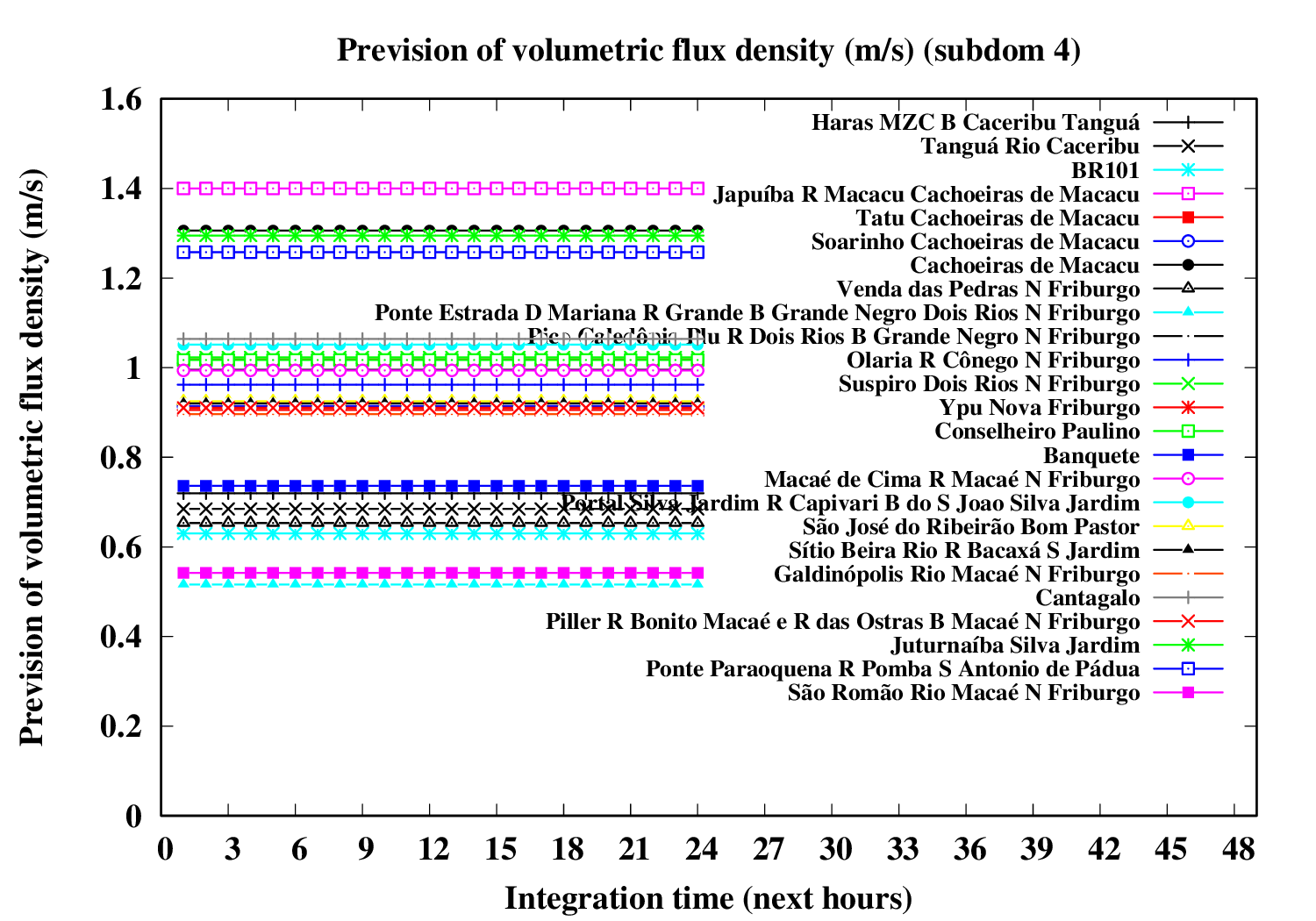
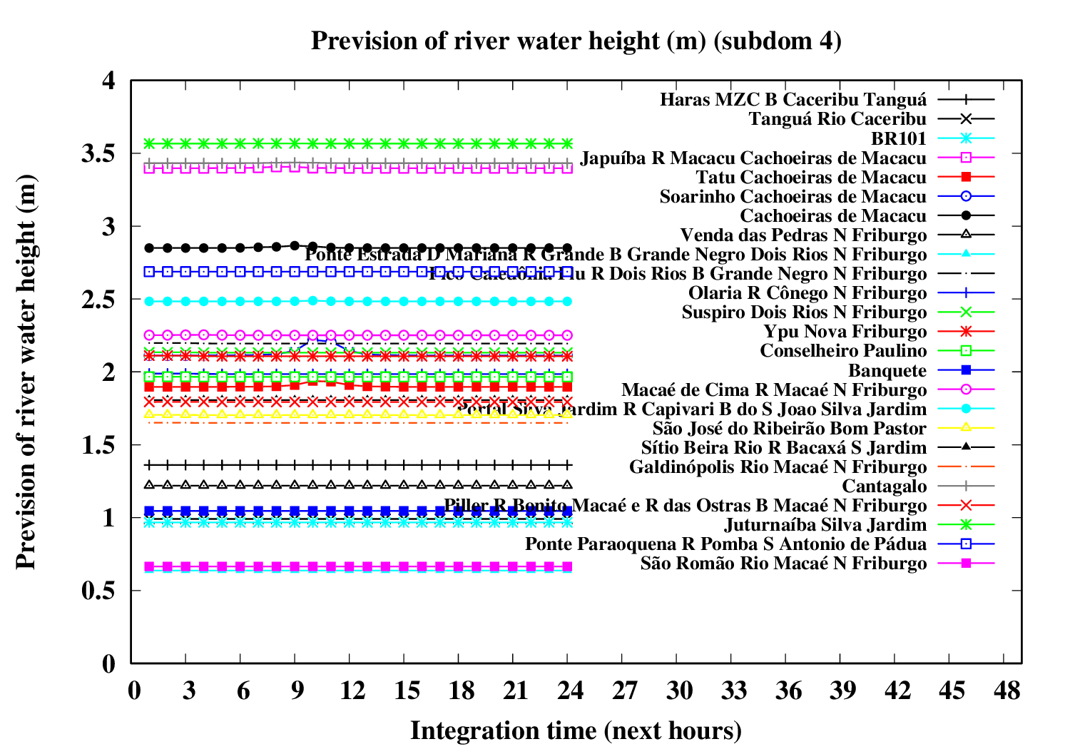
Subdomain 4:
| a) River water volumetric flux [Q] (m3 s-1) [next 24 hrs] | a) River water volumetric flux density [V] (m s-1) [next 24 hrs] | b) River water heigth [D] (m) [next 24 hrs] |
 |
 |
 |
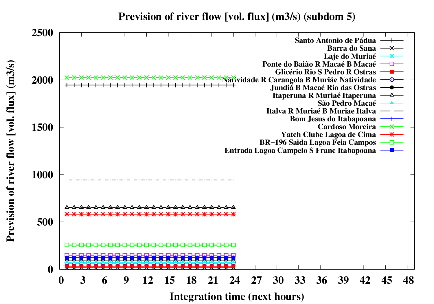
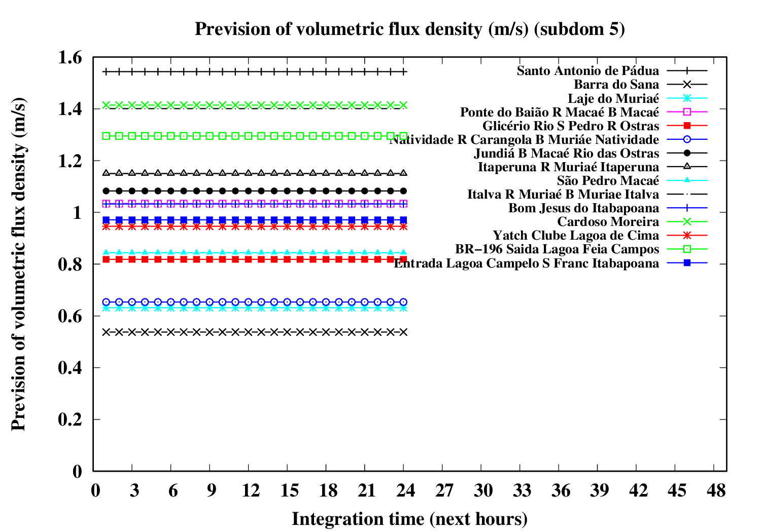
Subdomain 5 (eastward):
| a) River water volumetric flux [Q] (m3 s-1) [next 24 hrs] | a) River water volumetric flux density [V] (m s-1) [next 24 hrs] | b) River water heigth [D] (m) [next 24 hrs] |
 |
 |
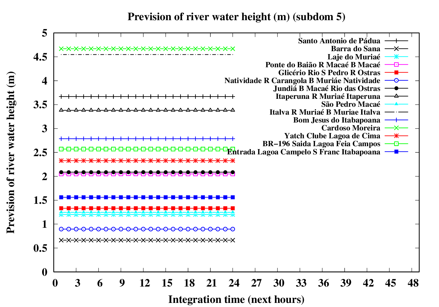 |
Variational modeling (24-hrs River Flood Nowcasting)
The evolution of river variables in the next 24 hours is obtained by coupling of the variational hydrologic model, the routing scheme based in displacement time interval of water parcels in excess by the surface and the river section model (that implements a river of trapezoidal section and inclined plainflood perperdicularly).
In the graphic, variable circle radius and translucent colors are proportional to the ratio between water deep and river bank height. An increase in the river flow (Q) implies increase both in flow velocity (V) and in water deep (D). If the water height excceds the riverbank height, occus overflow and overbank flood.The extension of floodplain depends of the excedence flow (Q) in relation to the river flow maximum capacity (i.e., Q > V W Dbank). A sucessive increase of the circle radius indicates increase in flood risk.
Five translucent colors are enough to update the flood risk every hour throughout the forecast period. Bright translucent circle colors are used and indicate the temporal evolution of river conditions throughout the forecast period, and are particularly variable in the sequence of rainy periods. A progressive color palette is applied, consisting of lime green, dark cyan, yellow, orange, red and violet. The predicted river overflow is indicated by violet circles.
| Status | Color | Range |
| Survelance | lime green | 0% ≤ D/Dbank < 50% |
| Warning | bright yellow | 50% ≤ D/Dbank < 80% |
| Alert | orange | 80% ≤ D/Dbank < 90% |
| High alert | vivid red | 90% ≤ D/Dbank < 100% |
| Overflow | violet (dark magenta) | 100% ≤ D/Dbank |
Animation: River Flooding Conditions [Nowcasting for the next 24 hrs]
| ... |
 |
Nowcasting of Precipitation Distribution
Advective rainfall predition (up to 3-hour in advance)
The very short-term forecast (one hour ahead) shown in the figures was obtained using an advection method. The advection method implements the estimation of steering flow based in the 2D advection partial differential equation. The sequence of the most recent precipitation fields along 24 hours (for each hour) are used to estimate the actual two-dimensional field of steering flow vector..
The first available approach method was to compute the steering flow by the velocity vector with components obtained by (cx, cy) = - ∂r/∂t [1/(∂r/∂x), 1/(∂r/∂y)]. This advective momentum estimation is similar the original approach proposed by Orlansky, them applied to advect perturbations across computational lateral boundaries in limited area numerical weather forecasting models. The actual implementation of the optical flow has three available mehods: Orlanski (1965), Horn and Schunck (1981) and Lucas and Kanade (1981), each one followed by a smoothing obtained by self-relaxation. The first method is local, the second variational iterative and the third direct. The sequence of optical flows every hour is obtained for the 24-hour period preceding the time of analysis. This sequence is used as input fields (observations) of the objective analysis obtained by Barnes interpolation (first, carried out over time and ultimately in space) (Barnes 1964; Koch et al. 1983). The resulting field preserves the macro-scale conditions of daily flow while is able to present the details associated with the optical displacement of the precipitating systems currently acting.
With these, it is possible to transport the precipitation field to the next hour, in a manner physically consistent with the timing of the precipitating system. Both local variation and structure transport are considered at each time step during the nowcasting period.
The methods available here for integration of the advection equation are: 1) the first-order Upwind Method (i.e., donnor cell method) (Hoffman and Frankel 2018, Mesinger and Arakawa 1976) and 2) the second-order Multidimensional Positively Defined Advective Transport Algorithm (MPDATA) (Smolarkiewicz 2006).
The next figure shows the 24-hrs recovered optical flow obtained by the method of Orlanski (1965), with pyramid strategy and Barnes interpolation through time and space.
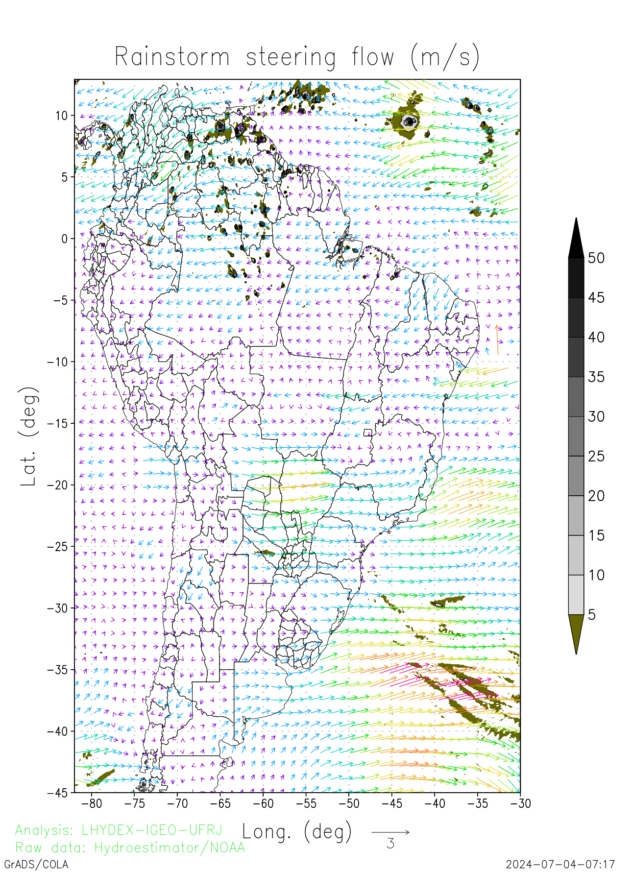 |
The advective optical flow is recovered at now based in the last 24 hours available fields. The structural data window correspond to the previous 24 hours (with 4 frames by hour).
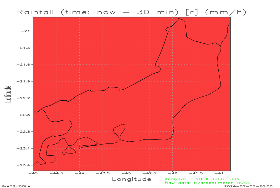
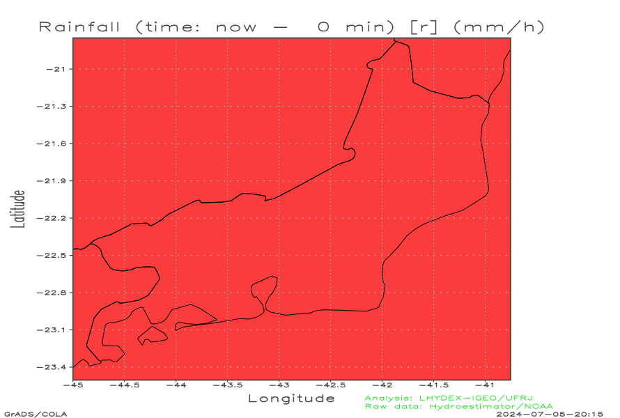
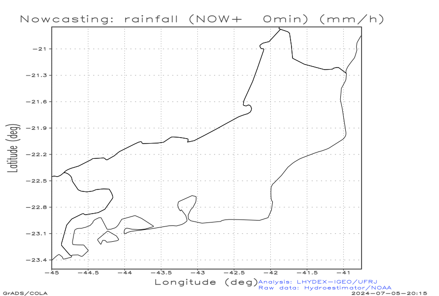
Rainfall fields to compute the advective optical flow in mesoscale
| Observed rainfall field r (mm h-1) (t - 30 min) | Observed rainfall field r (mm h-1) (t - 0 min) | Nowcasting rainfall field r (mm h-1) (t + 0 min) | |
 |
 |
 |
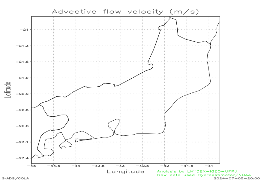
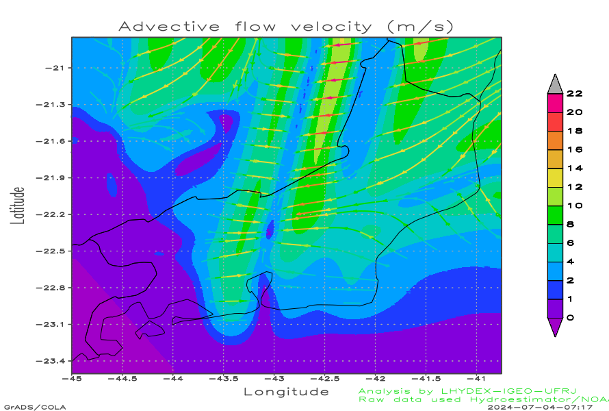
Regional advective optical flow (data window of 1 hour)
| 2D Advective flow (streamline) [time=Now-45 min] (m s-1) | 2D Advective flow (streamline) [time=Now-15 min] (m s-1) | 2D Acceleration (streamline) [time=Now-30 min] (cm s-1) |
 |
 |
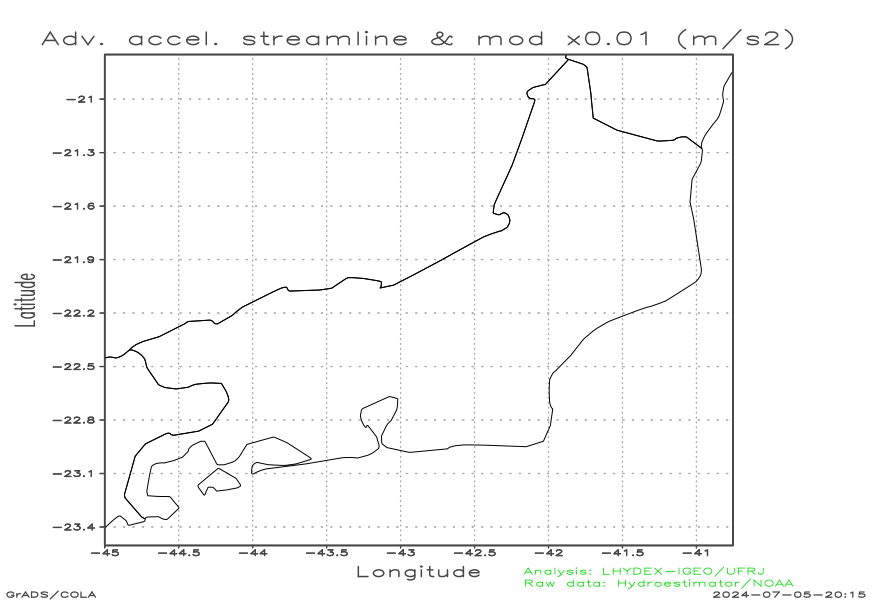 |
The local advective optical flow recovered with data of the previous 1 hour. The structural data window correspond to the previous 1 hour (with 4 frames by hour).
Advective nowcasting with optical flow (for the next 3 hours, outputs every 15 minutes)
Animation of the nowcasting fields: (a) rainfall [r] (mm h-1) and (b) radar refletivity parameter [dBZ] (dimensionless). Here the NWS-NOAA relation Z-R is applied, Z = 300 R1.4, instead the well known relationship Z = 200 R1.6 (Battan,1973), derived after the drop size distribution (DSD) of Marshall and Palmer (1948). The graphic presents the decibel of the modeled radar parameter Z, that is dBZ = 10 log10(Z/1), where the logarithm argument is the ratio between Z (mm6 m-3) and its unit scale.
The advective results below were obtained with the first-order Upwind Method.
| a) Nowcasting: radar refletivity parameter dBZ | b) Nowcasting: rainfall [r] (mm h-1) |
 |
 |
Nowcasting Check
As storms generally move from west to east, when evaluating the performance of advective nowcasting and persistence, only the eastern portion of the domain is relevant, since the advection time is sufficient for the storms to cross half of the zonal domain. Greater attention should be paid to the forecast starting 180 minutes ago (Figure in the lower right corner of the table ahead), comparing it with the current state. A positive dipole (from less to more flow down) centered on the centroid of the current storm indicates excess advective velocity, while a negative dipole (from greater value to smaller values in the direction of flow) indicates insufficient advective velocity. Thus, the advective velocity range can be finely adjusted using a tuning parameter in the advective program namelist.
Check of Advective Skill
The difference between the predicted and observed fields should result in aliasing, i.e., show an interference pattern with a spread-flange structure (i.e., with multiple ridges and valleys). The resulting image resembles the corrugated surface of cauliflower or a scrambled egg.
In this way, phase errors are reduced by modeled transport, relative to what would be possible by persistence.
Nowcasting Skill (precipitation diferences):
| Nowcasting skill: r(Nowcast)-r(Obs) (mm/h) [lag 15 min] | Nowcasting skill: r(Nowcast)-r(Obs) (mm/h) [lag 30 min] | Nowcasting skill: r(Nowcast)-r(Obs) (mm/h) [lag 45 min] |
 |
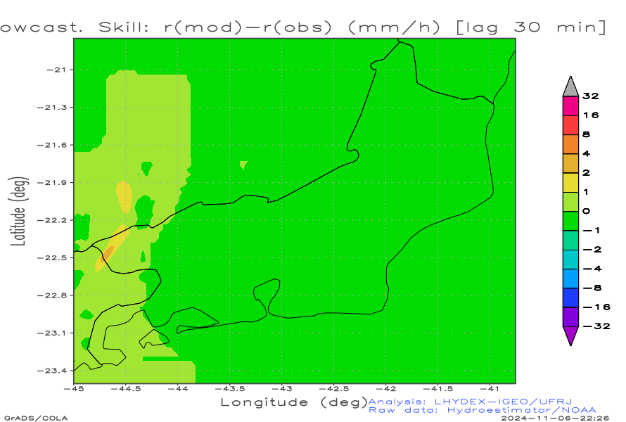 |
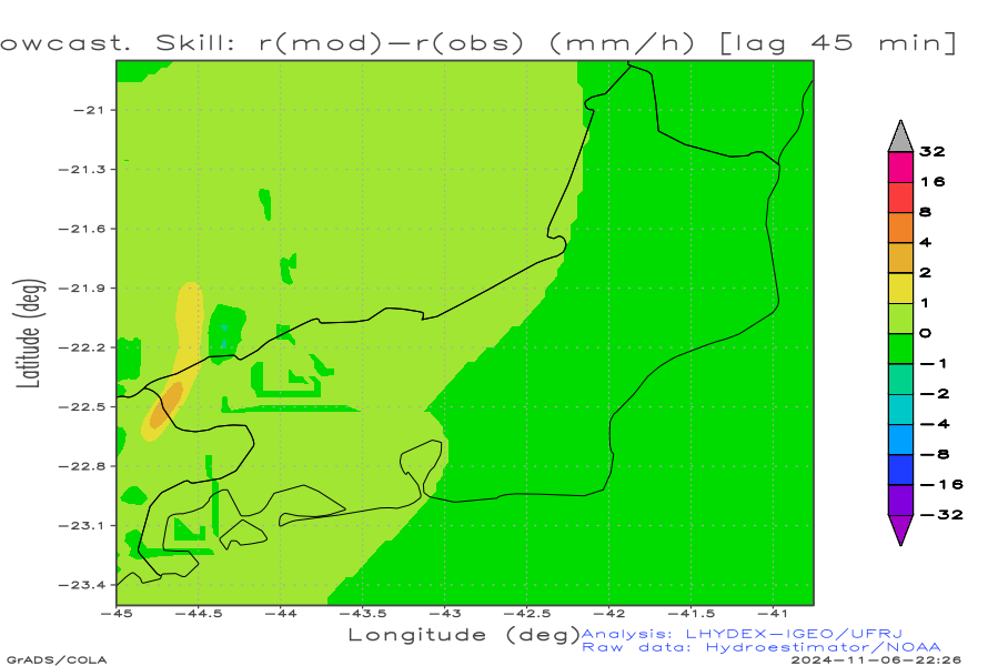 |
| Nowcasting skill: r(Nowcast)-r(Obs) (mm/h) [lag 60 min] | Nowcasting skill: r(Nowcast)-r(Obs) (mm/h) [lag 120 min] | Nowcasting skill: r(Nowcast)-r(Obs) (mm/h) [lag 180 min] |
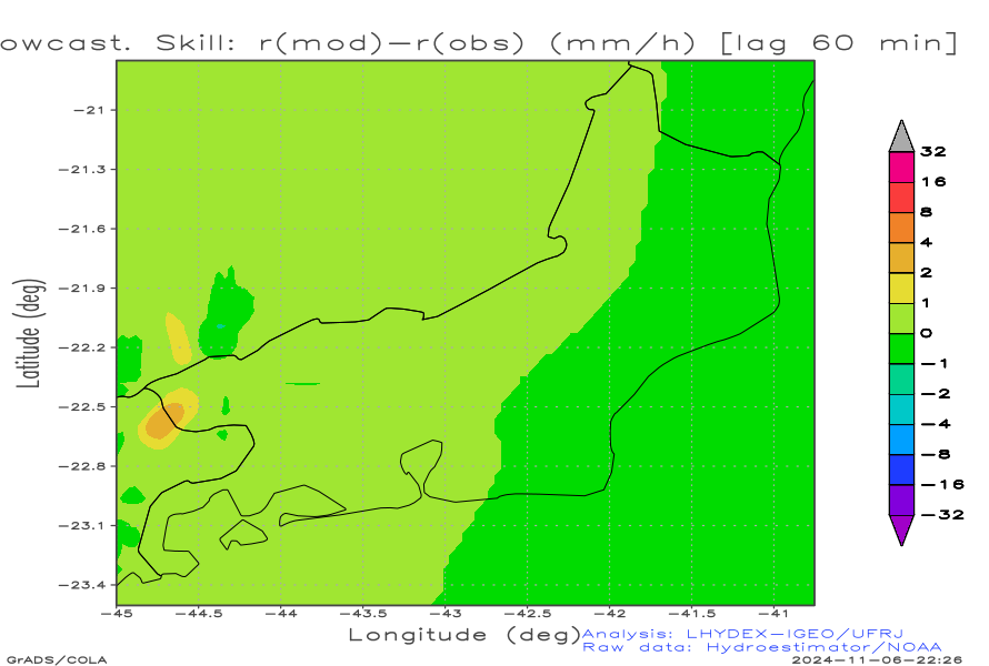 |
 |
 |
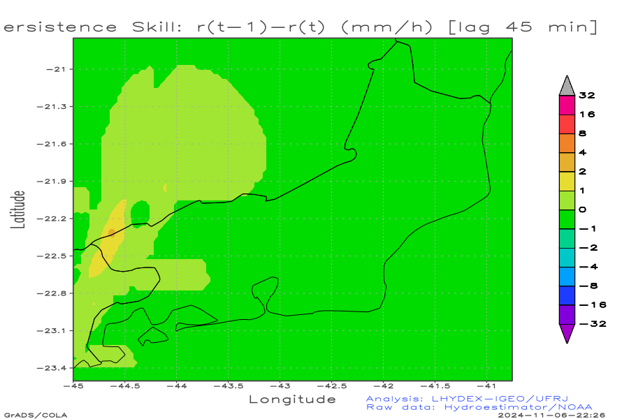
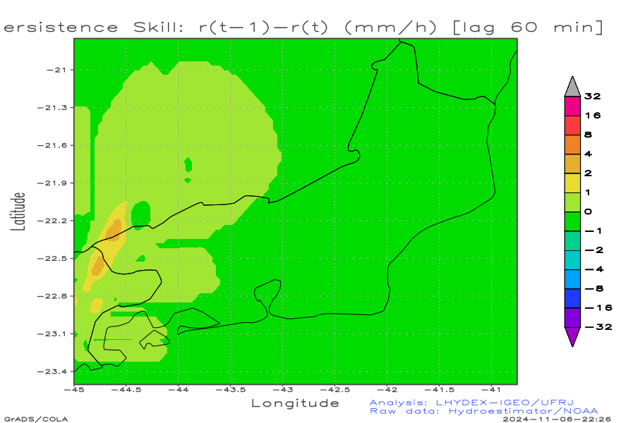
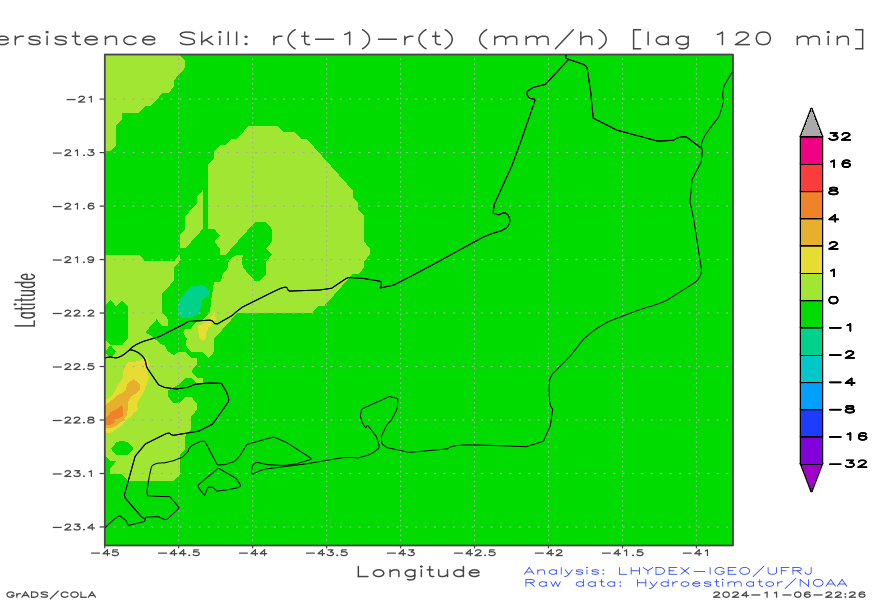
Check of Persistence Skill
The persistence method results in progressive separation of the fields as the forecast time interval increases. The resulting image resembles a puzzle that is unraveling.
Persistence Skill (precipitation diferences):
| Persistence skill: r(Persist)-r(Obs) (mm/h) [lag 15 min] | Persistence skill: r(Persist)-r(Obs) (mm/h) [lag 30 min] | Persistence skill: r(Persist)-r(Obs) (mm/h) [lag 45 min] |
 |
 |
 |
| Persistence skill: r(Persist)-r(Obs) (mm/h) [lag 60 min] | Persistence skill: r(Persist)-r(Obs) (mm/h) [lag 120 min] | Persistence skill: r(Persist)-r(Obs) (mm/h) [lag 180 min] |
 |
 |
 |
Nowcasting accuracy assessment
How is the advective optical flow velocity validated? As advective nowcasting advances in time, innovation (observation minus prediction) must be placed at the observation centroid. Thus, when positive [negative] innovation occurs (observation greater [less] than innovation) to leeward of the centroid, it indicates that the absolute velocity of the optical flow is underestimated [overestimated], and vice versa. Another way of saying this is to compare it with the temporal variation of innovation associated with the persistence method, in which the initial field is the forecast of future times. When advective transport generates results similar to persistence (but, in general, late [earlier] in relation to persistence innovation) it is a sign that the advective optical flow field presents underestimation [overestimation]. This allows for a (critical) assessment of the quality of the optical flow.
The precision and accuracy of the total storm variation rate is obtained by the numerical estimate of the total derivative, composed of the sum of the local variation of the advected (transported) field, from the previous observation to the present observation of precipitation, point by point of the grid used in the analysis and nowcasting. This assessment is important for the quality of nowcasting since it allows monitoring by advection of the total derivative, both the intensification and the decrease in precipitation of each individual storm, in the proposed nowcasting. In general, very intense and small storms show areas concentrated in a few contiguous grid points. In this case, the accuracy decreases rapidly with the advance of nowcasting in time.
In the first half hour, the very short-term forecast bias is estimated in relation to the maximum observed precipitation value, likely depending on the speed of movement, growth and dissipation of the storms. For nowcasting considering longer time intervals between forecast and observation, the bias increases more or less rapidly between half-hour and three-hour forecast. This loss of accuracy, represented by the increase in bias, may depend on the speed of precipitation development associated with the convective system, its spatial dimension, intensity and duration.
Commonly, the advective nowcasting gives more precision than the persistence, for the same forecast intervals. Therefore, in the advective method there is a progressive loss of statistical adherence of the predicted centroid in relation to the observed centroid, as long the convective systems move.
A relatively aliased spatial field, such as a field obtained by Laplacian smoothing is used to increase the accuracy of the estimates of the total variations with the spatial grid of discretization of the partial differential equation for conservative advection. Numerical truncation errors in the solution of the barotropic model for second order derivatives in large scale weather forecasting was discussed in 1970's and 80's by Shuman (1989).
Here, two steps are considered in nowcasting, a conservative step by the EDP solution of advection and a non-conservative step, associated with the variation in the precipitation rate of each convective cell, by estimating the total temporal derivative.
In other words, a generative [statistical] method for multiscale optical flow (arranged in Gaussian spaces or structured as Gaussian and Lagrangian pyramids) can be used to obtain "ensamble" sets of deterministic [optical advection] predictions . This allows evaluating the probability as the inverse of the variance of the forecast members at each new time. Not only innovation is obtained but also the probability of occurrence of precipitation, E(X). This is an important step in establishing a bridge with the real world of cost assessment (C for mitigation cust) and losses (L for probable loss) of risk analysis, since whenever the relationship (C/L) is less than E(X) mitigation actions are fully justified.
Additional comments on uncertainty
The advective method used in the nowcasting of the rain field presents two types of uncertainties, associated with i) position and ii) intensity. In fast moving rainfall fields, with transport speed equal to or greater than 10 m s-1, the nowcasting for the next 15 minutes can show a rainfall relatively small intensity compared with the observed one. The nowcasting intensity is near of 60% of the observed rainfall (firt order approach), mainly due to the Euler method (advanced in time) used in advection with time step of 1 second, and also, it is due to uncertainties of the precipitating system time in rapid evolution.
It is known the the thunderstorms presents three distinct phases of time evolution: 1) cumulus phase (rapid growth and predominant upward currents), 2) mature phase (precipitation of liquid water drops and hail, cloud electrification, gravity waves, upward and downward currents) and 3) dissipative phase (weak precipitation, downward movement).
Uncertainties in positioning produce phase errors (in relation to the maximum position or barycenter), producing dipole-type variations, up and down, around the barycenter and defining spindle rings around the neighborhood of the barycenter, commonly the maximum being better predicted. These distribution of positive and negative symmetric uncertainties, in the form of circular spindle sections, around the barycenter can indicate the effective nowcasting skill as a extrapolative transport method for nowcasting. For fields with little movement, with stationary barycenter (developing in a fixes positions in space), the evolution depends on the local derivative mainly, that is, on the intrinsic variation of the precipitating convective system over time. In this case, the intensity estimated by the advective nowcasting can be near to the persistence estimation.
One of the purposes of advective transport nowcasting is to reduce phase errors (i.e., position errors). To reduce nowcasting amplitude errors, a development submodel is needed for each Cumulus nimbus cloud that occurs during transport, as complementary processes. It should also be considered that convective systems are composed of different storms grouped into two subgroups, the first of storms in a mature phase and the second, of storms in dissipation, as shown by the former area development project called Thunderstorm Project in the mid-20th century.
How to interpret the results?
The graphs show:
- the spatial distribution of 24-hour cumulative precipitation over South America and coastal parts of the Atlantic (east) and Pacific (west) oceans;
- the animation of rainfall (mm h-1) made with 96 most recent frames, corresponding to the period of 24 hours prior to the current instant;
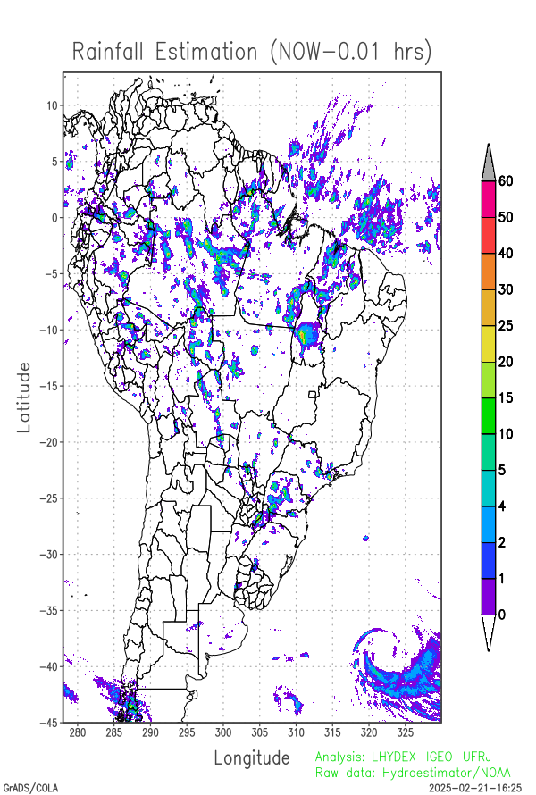
- the most recent field of estimated precipitation over South America by Hidroestimador / NOAA, built with the field of the last 15 minutes;
- the animation of rainfall (mm h-1) made with 12 most recent frames, corresponding to the period of 6 hours prior to the current instant;
- the rainfall hazard-risk index (mm2 s-1) and
- the hazard risk (%) obtained with the dynamic risk model based in soil field dynamics obtained by the numerical program TopModel_variational_f90_v2.**, coded in Fortran-90 (gfortran/linux)
- river forecast
- fields of advective speed of the precipitation field obtained by an optic flow method
- very short period forecast of precipitation for next 3 hours based in advective nowcasting by the optical flow, and
- nowcasting and persistence acuracies for precipitation rate (in the next three hours), considering bias (i.e., direct field differences.
The updating of the fields shown in the charts depends on data availability and uninterrupted online access. Occasionally, even with online access, there may be a service interruption for a few hours because servers may be restarting and updating during a planned outage. Therefore, continuity is not guaranteed. To work around this issue, mirrored web servers may become available in the future.
The results can be useful for meteorological research and also for assisting hydrometeorologists in the weather forecast centers during rapid evolution of rainstorms over prone risk areas (i.e., in nowcasting operations).
Examples of operational warning stages from a environmental risk in emergency management agencies
The Geo-Rio Foundation of the Municipality of Rio de Janeiro-RJ, Brazil (2020) uses operational warning stages to manage emergencies in the city of Rio de Janeiro, which are: normality stage, mobilization stage, care stage, stage alert and crisis phase.
The team from the Instituto Estadual do Ambiente (INEA) defined five stages for analyzing the risk of river flooding and flooding due to overflow of the banks of rivers in the State of Rio de Janeiro, in Brazil. The stage depends on the height of the water surface in the channel of each monitored river. The update takes place in minute cycles 24 hours a day for every day of the year, even holidays, directly from the situation room and hydrometeorological risk analysis: surveillance (no significant rain forecast that could cause river levels to rise), attention [i.e., warning] (possible rise in river levels due to rainfall), alert (above-normal rise of the level of a monitored river, with predicted elevation), high alert (imminent overflow of a monitored river, with forecast elevation), and overflow (record of the level of a monitored river above the overflow quota).
About the effect of rainfall remotion of atmospheric pollutants (Scavenging process)
Rain that crosses a polluted layer of the atmosphere removes gaseous and particulate pollutants by the Scavenging Process. The drops remove gases and particles of pollutants that are in their trajectories. Wet removal has a higher removal efficiency of air pollutants than dry removal (i.e., more efficient than the dry deposition associated with turbulent transport of pollutants in atmospheric boundary layer down to surface). The deposition transfers air pollutants from the atmosphere to the surface elements (i.e., to the vegetation surfaces, bodies of water etc). Once transported to the surface, pollutants can be sedimented, chemically and physically transformed by absorption and / or absorption.
Biosphere beings also absorb pollutants, such as plants and animals. Plants in particular absorb pollutant gases by removing them from the atmosphere either by the plant epidermis or through small structured openings of cells called stomata, which are biophysically controlled, opening for photosynthesis and respiration. The pollutants thus can thus pass to the animals by feeding (i.e., following the ecological chain). This is critical in the case of surface areas contaminated by radionuclides and heavy metals.
The pollutant present in the rainwater can infiltrate the soil, crossing the different layers of soil, reaching the water table and even the aquifer in the most severe case. Thus, pollutants in the water can be transported in the superficial and subsurface flows (which make up the runoff), until reaching different bodies of water, such as lakes, rivers, mangroves, deltas, estuaries, bays towards the largest bodies of water (ie, seas and oceans).
About the hydro estimator of precipitation
The graphs above show results obtained from online available Hydroestimator/NOAA/USA dataset of the last 24 hours. The hydroestimator/NOAA methodology estimates the convective precipitation using a ratio between the brightness temperature of the top of convective clouds (storms) and the atmospheric precipitation at the surface. The gross irradiance data comes from geostationary GOES series satellites (Scofield 1987; Vicente et al. 1989; Field and Menzel 1998; Scofield and Kuligowski 2003).
In perspective
It is considered to inform the nowcasting system with joint precipitation analysis based on assimilation of lightning data with a high sampling rate, for example, from lightning data from the GOES-R satellite ( 2018).
Acknowledgments
Thanks to NOAA/STAR for providing public access to Satellite Convective Precipitation Estimation (GOES) (Hydro-Estimator) fields, which are used by lhydex-UFRJ to define the initial conditions of nowcasting and to diagnose hydrometeorological hazards in cycles of rapid update.
Bear in mind that
The results presented on this site are experimental and their use is the entire responsibility of the user.
Attention: disclaim statement
This project is experimental. We continually check and evaluate the use and performance of the system made available to multiple users. We also continuously check the loading of source data, the production of images, graphics and aminations, the (over)loading of the operational computers and the status of the web servers used. The products presented in this project cannot be used for commercial purposes, unless the user has written authorization from the person responsible for the Experimental Hydrometeorology Laboratory at UFRJ (lhydex-UFRJ). The lhydex-UFRJ laboratory does not give any guarantee regarding these products. In no case will lhydex-UFRJ be liable for special, indirect or consequential damages, or any damage linked to or arising from the use of these products. Furthermore, lhydex-UFRJ cannot guarantee the regularity of these products.
Copyright
All materials shown on this website are authored by the laboratory coordinator, unless otherwise indicated. The use of this content is free for purposes of learning, study and technical-scientific improvement, as long as it cites the source reference. The content in this site is for education and non commercial use only. Banned for commercial use.
Post Address
Laboratório de Hidrometeorologia Experimental (lhydex-UFRJ)Departamento de Meteorologia, Instituto de Geociências
Centro de Ciências Matemáticas e da Natureza
Universidade Federal do Rio de Janeiro - IGEO-CCMN-UFRJ
Av. Athos da Silveira Ramos, 274, Cidade Universitária
Rio de Janeiro, RJ, Brasil, CEP 21941-916
Contact
E-mail link: Send Mail
Bibliography
- Barnes, S.L. 1964, A technique for maximizing details in numerical weather-map analysis. Journal of Applied Meteorology, vol. 3, no. 4, pp. 396–409. Web link.
- Battan, L.J. 1973, Radar Observations of the Atmosphere. Univ. of Chicago Press, Chicago, USA, 324 p.
- Beven, K.J. 2000, Rainfall-runoff modelling. The Primer. Wiley, 360 p.
- De Blasio, F.V. 2011, Introduction to the physics of landslides. Springer, 408 p.
- Farr, T.G. et al. 2007, The Shuttle Radar Topography Mission, Rev. Geophys., vol. 45, RG2004, doi:10.1029/2005RG000183.
- Field, Menzel, W.P. 1998, The operational GOES infrared rainfall estimation technique. Bull. Amer. Meteor. Soc., vol. 79, pp. 1883-1898.
- Horn, B.K.P. & Schunck, B.G. 1981, Determining optical flow. Artificial Intelligence, vol. 17, pp 185–203. Web link.
- Kirkby, M.J. 1998, TopModel: A Personal View. In: Beven, K.L.(Editor): Distributed Hydrological Modelling: application of TopModel concept. pp. 19-29. Series: Advances in hydrological processes. Web link.
- Koch, S.E., DesJardins, M., Kocin, P.J. 1983, An interactive Barnes Objective Map Analysis Scheme for Use with Satellite and Conventional Data. Journal of Applied Meteorology and Climatology, vol. 22, no. 9, pp. 1487-1503. Web link.
- Hoffman, J.D. & Frankel, S. 2018, Numerical methods for engineers and scientists. CRC press. 825 p.
- Liu, G., Schwartz, F. W., Tseng, K.-H. and Shum, C. K. 2015, Discharge and water-depth estimates for ungauged rivers: Combining hydrologic, hydraulic, and inverse modeling with stage and water-area measurements from satellites, Water Resour. Res., vol. 51, pp. 6017–6035, doi:10.1002/2015WR016971.
- Lucas, B.D., Kanade, T. 1981, An Iterative Image Registration Technique with an Application to Stereo Vision. In the Proceedings of Imaging Understanding Workshop, pp. 121-130, lucas_bruce_d_1981_2.pdf.
- Marshall, J.S., Palmer, W.McK. 1948. The distribution of raindrops with size. Jounal of Meteorology, vol. 5, pp. 165-166.
- Mesinger, F., Arakawa, A. 1976, Numerical methods used in atmospheric models. WMO publication, GARP PUBLICATIONS SERIES No. 17, 70 p.
- Orlanski, I. 1965, A simple boundary condition for unbounded hyperbolic flows. Journal of computational physics 21, no. 3 (1976): 251-269. orlanskiJCP1976.pdf.
- Smolarkiewicz, P.K. 2006, Multidimensional positive definite advection transport algorithm: an overview. International journal for numerical methods in fluids, vol. 50, no. 10, pp. 1123-1144.
- SRTM-NASA, SRTM website link, viewed Dec 2020.
- Rodriguez, E., Morris, C.S., Belz, J.E., Chapin, E.C., Martin, J.M., Daffer, W., Hensley, S. 2005, An assessment of the SRTM topographic products, Technical Report JPL D-31639, Jet Propulsion Laboratory, Pasadena, California, 143 p. SRTM_paper.pdf.
- Scofield, R.A. 1987, The NESDIS operational convective precipitation estimation technique. Mon. Wea. Rev., vol. 115, pp. 1773-1792.
- Scofield, R.A., Kuligowski, R.J. 2003, Status and outlook of operational satellite precipitation algorithms for extreme-precipitation events. Mon. Wea. Rev., vol. 18, pp. 1037-1051.
- Shuman, F.G. 1989, History of Numerical Weather Prediction at the Nacional Meteorological Center. Weather and Forecasting, vol. 4, pp. 286-296.
- Vicente, G.A., Scofield, R.A., Menzel, W.P. 1998, The operational GOES infrared rainfall estimation technique. Bull. Amer. Meteor. Soc., vol. 79, pp. 1883-1898.
- GOES-R Algorithm Working Group and GOES-R Series Program 2018, NOAA GOES-R Series Geostationary Lightning Mapper (GLM) Level 2 Lightning Detection: Events, Groups, and Flashes. [indicate subset used]. NOAA National Centers for Environmental Information. doi:10.7289/V5KH0KK6. [access date].